Two systems, coupled only at the coil

In most existing buildings the chilled water and heating hot water plants are hydraulically independent and meet only at the air handler coils, so the conventional MEP process sizes and designs each one on its own.

Electrification changes that at sites with significant coincident load: university campuses, hotel and casino precincts, airports, convention centres and hospitals. A chiller at a COP of 5 rejects 1.2 kWh of heat at the condenser for every kWh of cooling, and on these sites the boilers are often heating the same buildings at the same time. Heat recovery chillers, water source heat pumps and thermal storage let a coupled plant move that heat instead of generating it.

Coupling also removes the separability that the conventional process depends on:

• Capacity becomes interdependent: the heat a recovery machine can deliver depends on the cooling load at that instant.
• Storage couples the plant across time: chilled water made at the 8 am heating peak can serve the 3 pm cooling peak.
• Supply temperature couples the plant to the coils: heat pump capacity and COP depend on the supply temperature the existing coils need.
• Performance depends on dispatch: the same equipment under a different control policy uses a different amount of energy.

A design-day calculation cannot represent any of these. A coupled, electrified plant has to be simulated to be designed.

The same problem we solve in controls

Our controls work fits a performance model to each machine from the plant's own trend data: COP as a surface over load and lift. We combine those into a plant model and solve offline for minimum total plant power at every combination of load, wet bulb and stage, within surge, choke, flow and manufacturer limits. The incumbent controls contractor implements the result in the existing BMS as an explicit control law.

That is the structure of explicit model predictive control (MPC): a constrained optimisation solved once, offline, across the parameter space, then evaluated online as a lookup (Bemporad, Morari, Dua and Pistikopoulos, Automatica, 2002).

Plant design has the same structure, one level up. Machine types, capacities and storage become the decision variables, a measured year of load and weather becomes the parameter set, and capital cost, 20-year cost, emissions, peak demand and machine run hours become the objectives.

Two differences make the design problem harder

The first is that design is a bilevel problem: the outer loop chooses the plant, and the inner loop chooses how to operate it. Each candidate has to be scored under its own optimised dispatch, or the comparison ranks control strategies rather than plants. The controls optimisation becomes a subroutine of the design optimisation.

The second is that storage and staging make the inner problem dynamic. State of charge, minimum run and off times and cycle-rate limits link each interval to the next. A design simulation that dispatches storage with a fixed rule, or ignores cycling, will misvalue the tank and missize the machines, and that is usually where the largest capital trade-offs sit.

We call this approach model predictive design (MPD). MPC predicts how a plant will respond and chooses the actions that optimise that prediction. MPD predicts how each candidate plant will perform over a measured year and across uncertain futures, with its own optimised control running inside every prediction. A controller revisits its decision every few minutes. A design decision lives for 20 years, which is the argument for spending more on the prediction.

The solution space for a retrofit

For an existing chiller and boiler plant, the design variables fall into a natural order. Recover first: heat recovery chillers and water source heat pumps sized against the coincident load, with storage to bridge the daily offset between the peaks. Then add a second source, usually air-source heat pumps, for heating with no concurrent cooling, and decide whether the boilers stay on standby. Then a low-load chiller, the machine split and redundancy.

The constraints are physical: roof area, plant room height, structure, the supply temperature the existing coils accept, zero unmet hours on the worst measured day, and electrical supply, because heating that arrived by gas main now arrives by switchboard.

Three heat pump manufacturers, three capacity splits, three sizes for each of three stores and a low-load chiller or not give 486 combinations, before any capacity is treated as continuous. A spreadsheet can compare five options. It cannot search this space.

Model predictive design is scoped to energy, emissions and cost. Vibration, acoustics, structure, hydraulics, refrigerant safety and code compliance remain with the consulting engineer.

Parameterise the model from measured load

The core input is twelve months of heating and cooling delivered, at hourly resolution or finer. The key derived quantity is the coincident load, the smaller of heating and cooling at each instant:

L_c(t) = min( H(t), C(t) )

Here is how that parameterises the model on an example university campus in Sydney. The charts use representative data to aid the description of each stage in the design process. It delivers about 17 GWh of cooling and 13 GWh of heating a year, with both peaks close to 8 MW.

‍

‍

Each statistic sets a bound for the first search stage:

• Annual coincident load is 7.8 GWh, 60% of annual heating. This is the upper bound on recoverable heat, before lift and losses.
• Non-coincident heating is 5.2 GWh, almost all of it between April and October. This sizes storage and the second source.
• The intraday offset is about eight hours in every season: heating peaks around 07:30 as buildings warm up, and cooling around 15:30.
• On the 95th percentile day, about 50 MWh of heating has no concurrent cooling, the upper bound on useful storage energy. Tank volume is cheap per MWh and expensive in floor area, air source capacity is cheap in floor area and expensive in peak demand, and the tariff decides where the crossover sits.

‍

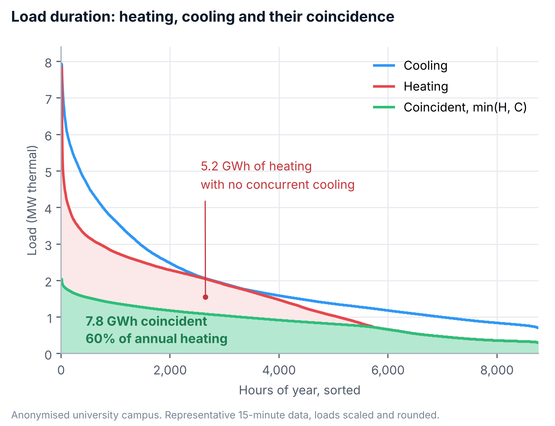
Each statistic sets a bound for the first search stage:

• Annual coincident load is 7.8 GWh, 60% of annual heating. This is the upper bound on recoverable heat, before lift and losses.
• Non-coincident heating is 5.2 GWh, almost all of it between April and October. This sizes storage and the second source.
• The intraday offset is about eight hours in every season: heating peaks around 07:30 as buildings warm up, and cooling around 15:30.
• On the 95th percentile day, about 50 MWh of heating has no concurrent cooling, the upper bound on useful storage energy. Tank volume is cheap per MWh and expensive in floor area, air source capacity is cheap in floor area and expensive in peak demand, and the tariff decides where the crossover sits.

‍

These bounds become the box constraints on the search.

Trial lower supply temperatures through a winter

Supply temperature sets the sink side of every heat pump's lift. For a heat pump drawing heat from 77°F (25°C) condenser water, dropping the supply temperature from 176°F to 158°F (80°C to 70°C) cuts the lift from 99°F to 81°F (55 K to 45 K) and raises the ideal (Carnot) heating COP by about 19%. Real machines differ from Carnot, but the direction holds, and some cannot reach 176°F (80°C) at all at low source temperatures.

Most existing boiler plants run at 176°F (80°C) because they always have. This is a question to answer in the field, not in a simulation. Before electrifying, reset the existing boilers to 167°F (75°C) and then 158°F (70°C) across a winter, trending zone temperatures and valve positions through cold mornings and warm-ups.

Valves at 100% with zones below setpoint mark the coils that limit the reset. Upgrading those coils then goes into the design as a capital line item rather than a surprise after the heat pumps arrive.

SIFT: wide, then deep

Every simulation trades precision against the number of evaluations. SIFT is how we carry out model predictive design in practice, in four stages: Screen, Iterate, Fit, Test. The principle is wide, then deep: spend computation on breadth while it is unclear where the good region of the solution space is, and on depth once the decision is close.

Screen. About 1,000 permutations, sampled across the bounds set by the load data. Every machine has a constant efficiency and an on/off state, the time step is hourly, and dispatch follows a fixed merit order: recover, discharge storage, air source, then boilers. The model is deliberately crude. It shows at low cost which axes the answer is sensitive to and which regions are dominated.

Iterate. About 100 designs per round, with the bounds narrowed around the non-dominated set after each round. COP now depends on lift, and state of charge is tracked hourly, giving a credible daily energy consumption and storage cycle for each design.

Fit. About 10 candidates, built from real equipment. We fit three-dimensional performance surfaces (COP against load fraction and lift) to manufacturers' part-load data and calibrate retained machines to their own record. The time step drops to 15 minutes, staging and storage rate limits are modelled, and each candidate gets its own optimised dispatch: the controls optimisation running as the inner loop. It returns system COP, run hours and starts per machine, cycling and unmet hours. This is the stage where right-sizing happens.

Test. Two or three candidates, run through a Monte Carlo analysis of the inputs nobody can measure.

‍

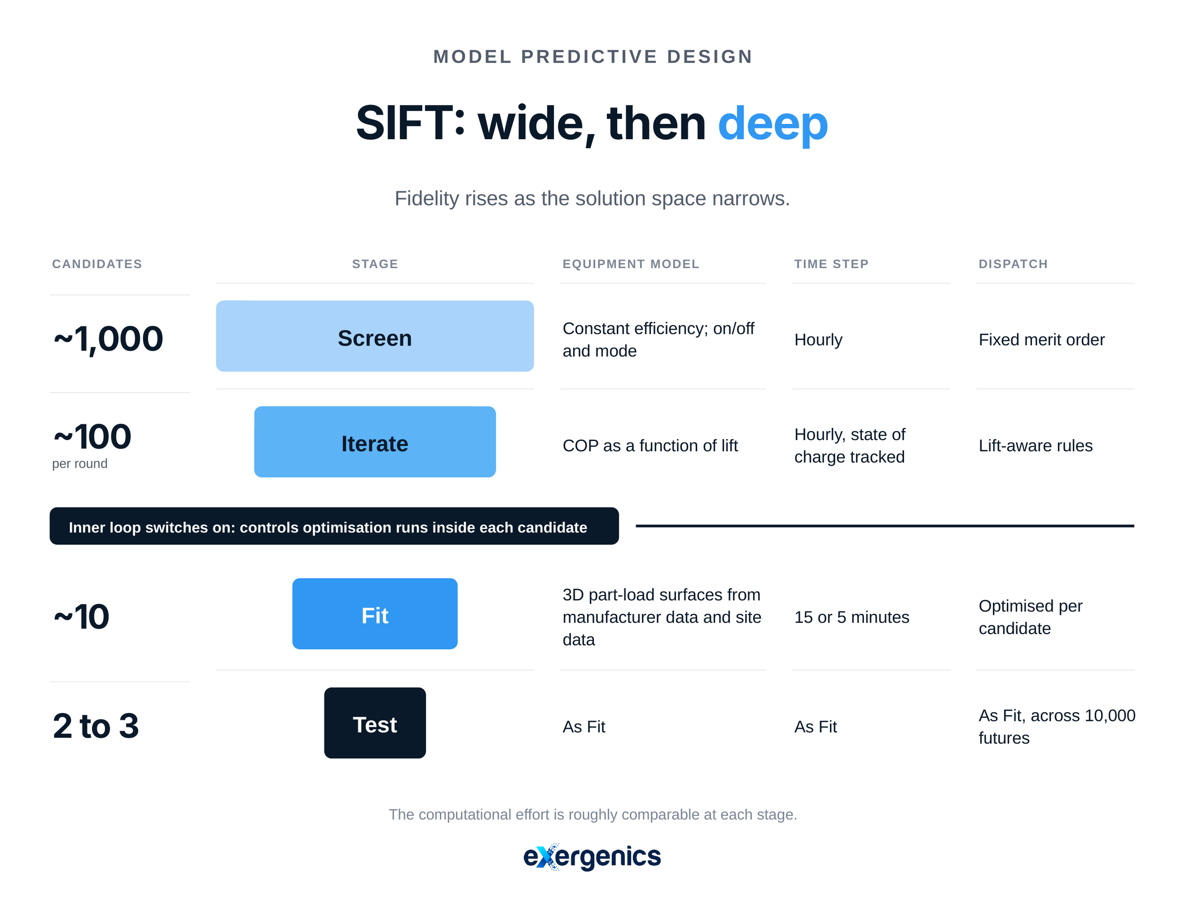
Each stage scores several objectives at once, so the result is a Pareto frontier rather than a single answer. The frontier is ours to produce. The point on it is the owner's to choose.

Test: how often is it the best design?

A single 20-year figure assumes one future. The inputs that decide the ranking are uncertain: future load, energy price and tariff shape, the grid emissions trajectory, carbon and offset prices, and refrigerant leakage. Each design is exposed to them differently. A design weighted toward air source capacity is more exposed to tariff shape; one weighted toward storage is more exposed to whether the measured load profile holds.

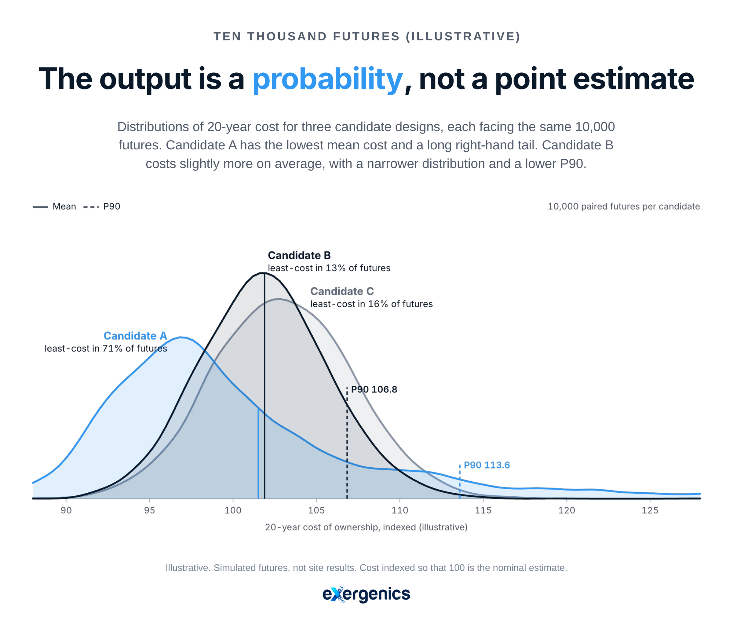
The Test stage samples 10,000 futures, and every candidate faces the same 10,000, so differences between candidates reflect the designs and not sampling noise. The outputs are the probability that each candidate is the least-cost option, the expected regret of choosing each one, and which input drives the ranking when it changes. If two candidates swap places depending on one input, that input is the one to work on.

The candidate with the lowest mean cost is not automatically the one to choose. A candidate with a slightly higher mean and a much narrower upper tail carries less exposure to the futures an owner would least like to face, and some owners will rightly pay for that.

‍

The design sets the controller's feasible set

The reason for the Fit stage is what happens when the design is wrong. A controller optimises within the feasible set the plant defines. A poorly sized plant leaves the controller choosing the best option from a poor set.

Here is an example from twelve months of 15-minute data at a large entertainment venue (capacity, machine count, building type and location changed; load ratios as measured, rounded).

‍

Installed cooling capacity is about 18 MW across five machines. Peak demand, excluding transients after stage changes, is just under 40% of installed capacity. The median load while running, across more than 5,000 hours, is about 5%. The low-load machines have run roughly eight times the hours of the high-load machines.

We simulated about 60 staging strategies on the plant's own data. The one that equalises runtime as far as control allows still leaves a gap of about 1,000 hours between the low-load and high-load machines, and costs close to 2% of plant efficiency every year for the life of the asset. Control chooses which machines run. It cannot change which machines were bought.

A coupled, electrified plant has more ways to go wrong, and each shows up in Fit-stage run hours and starts per machine before the equipment is ordered.

If you're evaluating a concept design or pre-feasibility options for a precinct electrification project, we can run a Screen-stage analysis on your site's trend data. Contact us here.

If you have designed or commissioned a coupled heat recovery plant, we'd like to hear how it performs against its model. Either way, send us an email. We read every one.

Iain Stewart

Cofounder & CEO, Exergenics

www.exergenics.com

‍

‍

‍

‍